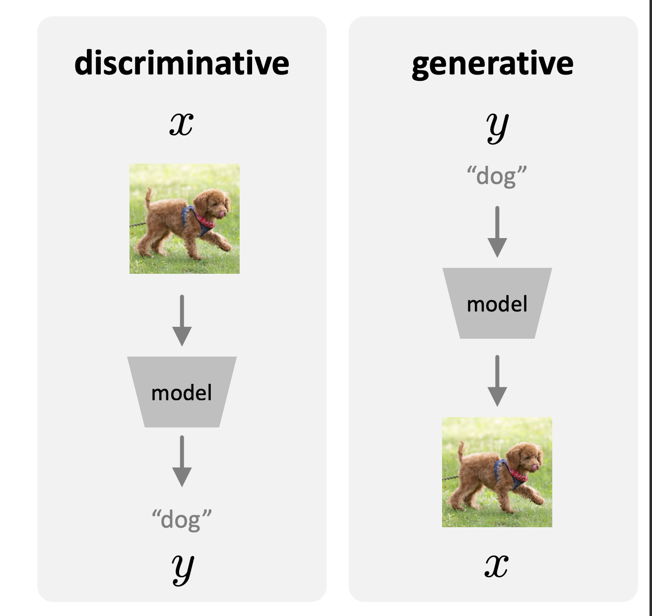
The rise of large models has advanced the way of how we move towards to the intelligence. In the past decades, people worked on “discriminative” intelligence, that is, we predict a dog image as a “dog”. To do so, we train on a batch of dataset containing different categories with labels, and train with the goal that every output matches the corresponding classes. The great success of LLM has brought us into a new era: GenAI. Unlike the discriminative model, we generate the image “dog” given the input prompt (text, image, …). This is called generative model.
A generative model can have multiple possible outputs and some predictions are more plausible than some others. At the same time, predictions can be more complex, more informative, and higher-dimensional than the input. Suppose the “label” is $y$, and the sample is $x$, we have $$ p(y|x) = p(x|y) \frac{p(y)}{p(x)}. $$ This is the Bayes’s rule. $p(x|y)$ means given the $y$, the possibility of $x$, which represents the generative results. Rather, $p(y|x)$ represents the discriminative results given $x$. For a generative problem, we can assume we know $p(x)$, and $p(y)$ is also known prior. Then we can find the generative models can be discriminative. Conversely, given the discriminative model $p(y|x)$, to make it generative, we still need to model the distribution of $x$.
As shown above, generation is about probability as probability represents different data distributions. And at the core of the generative models are the modeling of the distributions. An intuitive way is to get a set of distribution of every samples. Yet we will soon find that it far exceeds the computational ability. And an “exact” depiction of the distribution will lead to the overfit to one specific distributions.
 Therefore, as shown above, we want to learn a probability distribution $p(x)$ that
- Sampling: If we sample $x_{\text{new}} \sim p(x)$, it should look like a “dog”
- Density Estimation: $p(x)$ should be high if $x$ looks like a dog, and low otherwise
- Unsupervised Learning: We should model $p(x)$ as what it is common
Therefore, here is the process. We have a dataset $x^{(t)}$, and actually the distribution of the data is objective. And we estimate the distribution using analytical forms or neural networks. Then the goal is to optimize the “distance” of the two distributions. At the inference stage, we sample from the learnt distribution given $y$, which is $p(x|y)$. To some extent, generative models are about $p(x|y)$.
This is the general idea of generative models. And at this stage, we can ask the following questions:
- How to formulate the problem as a probabilistic modeling and decompose complicated distributions into simple and traceable ones?
- How to measure the “distances” between the distributions?
- How to model/represent the data distributions?
- How to learn/optimize/train the problem?
- How to do the inference (sample, density estimation)? This is a basic road map of the deep generative model. Before we start to go through different models, we should take some steps at how we should measure the “distance”, i.e. how should we learn the generative models in a general way.
Maximum Likelihood Learning
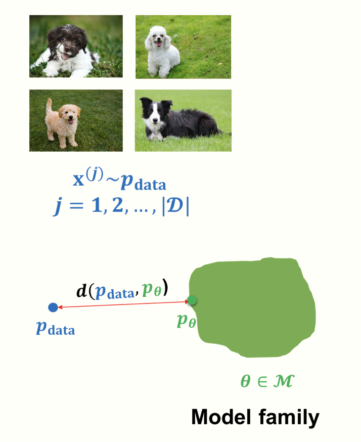
We assume there is a distribution $P_{data}$, and a dataset $\mathcal{D}$ of $m$ samples from $P_{data}$. The standard assumption is that the data instances are independent and identically distributed (IID). The goal of the learning is to return a model $P_{\theta}$ that precisely captures the distribution $P_{data}$ from which our data was sampled. However, this is generally not achievable because we only have limited data, which only provides a rough approximation of the true distribution and the computation resources is overwhelmed. Therefore, a compromised way is to train a neural network, that has the most “closest” distribution. Then the question becomes: how can we measure the closeness? To answer this question, we resort to KL divergence, which is given by $$ D(p(x)||q(x)) = \sum_{x} p(x)\log \frac{p(x)}{q(x)}. $$It has several properties. First, $D(\cdot || \cdot) \ge 0$ for all distributions $p$ and $q$, with equality iff $p=q$. Therefore, if we consider $p$ as the true distribution, and $q$ as the distribution model learns, the larger the differences, the higher of KL-divergence. Intuitively, if the data comes from $p$, but we use a scheme optimized for $q$, the $D$ measures how many extra bits (information) we need on average. In other word, it measures the “compression loss” of using the predicted models, which is in alignment with our designing goals. Note that KL-divergence is asymmetric, meaning that $D(p||q) \ne D(q||p)$. Then how to assign $p$ and $q$ with the true and predicted distribution is worth discussing. In Maximum Likelihood Estimation (MLE) learning, we adopt the following form,
$$ \begin{aligned} D(P_{data}||P_{\theta}) &= \sum_{x} P_{data}(x) \log\frac{P_{data}(x)}{P_{\theta}(x)} \\ &= \mathbb{E}_{x \sim P_{data}}\left[\log \frac{P_{data}(x)}{P_{\theta}(x)}\right] \\ &= \mathbb{E}_{x \sim P_{data}}\log[P_{data}(x)] - \mathbb{E}_{x \sim P_{data}} \log[P_{\theta}(x)] \end{aligned} $$
The second line uses the trick $\sum_{x} p(x) q(x) = \mathbb{E}_{x \sim p(x)} q(x)$.
$x \sim p(x)$ means samples from distribution $p$. Let’s take a look at the third line.
The first item does not depend on $P_\theta$, a.k.a. the constants. And if we want to minimize the KL divergence, we can equivalently maximizing the expected log-likelihood, i.e.,
$$ \arg \min_{P_{\theta}}D(P_{data}||P_{\theta}) = \arg\max_{P_{\theta}} \mathbb{E}_{x \sim P_{data}} \log[P_{\theta}(x)]. $$
Intuitively, the maximum of likelihood estimation gives us: maximize the probability of the data given specific parameters. Given the data, the likelihood function is given by the product of the probability. And the product can then be computed as the summation of the log function. Therefore, by maximizing the log-likelihood, we can find the most “reasonable” contributions. Note that we “sample” from the distribution, and we use the sampled average as the expectations. It is Monte Carlo Estimation. The approximated version of the expectation is $$ \mathbb{E}_{x \sim P_\text{data}}[\log P_\theta(x)] \approx \frac{1}{N} \sum_{i=1}^N \log P_\theta(x_i). $$
Monte Carlo Estimate is an unbiased estimation. Here is a proof. Given a expection
$$ I = \mathbb{E}_{x \sim p(x)} [f(x)] = \sum_{x} p(x)f(x), $$
we get the Monte Carlo Estimation:
$$ \hat{I} = \frac{1}{N} \sum_{i=1}^{N} f(x_i). $$
Then we have
$$ \mathbb{E}[\hat{I}] = \mathbb{E} \left[ \frac{1}{N} \sum_{i=1}^{N} f(x_{i})\right]= \frac{1}{N}\sum_{i=1}^{N} \mathbb{E}[f(x_{i})] = I. $$
By now, we have introduced the basic idea of learning a generative model by using KL-divergence as the learning metrics. In the next, we will introduce the most popular generative modeling nowadays.
Autoregressive Modeling
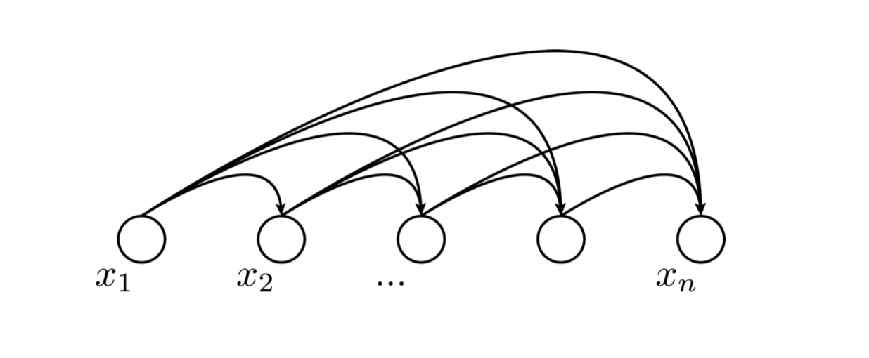
Let’s start from the joint representation. Any joint representation can be written as a product of conditionals in any order and partition. Suppose we have the data $x_{1}, x_{2}, \cdots, x_{n}$, we can model the joint distribution as
$$
p(x_{1}, x_{2}, \cdots, x_{n}) = p(x_{1})p(x_{2}|x_{1})\cdots p(x_{n}|x_{1}, x_{2}, \cdots x_{n-1}).
$$
The most straightforward means is to represent every conditional probabilities as a table, which is obviously too time-consuming. And if we make use of the representation abilities of neural networks, we can similarly model every conditions as a neural network, that is
$$
p(x_{1}, x_{2}, \cdots, x_{n}) = p_{\theta}(x_{1})p_{\phi}(x_{2}|x_{1})\cdots p_{\Phi}(x_{n}|x_{1}, x_{2}, \cdots x_{n-1})
$$
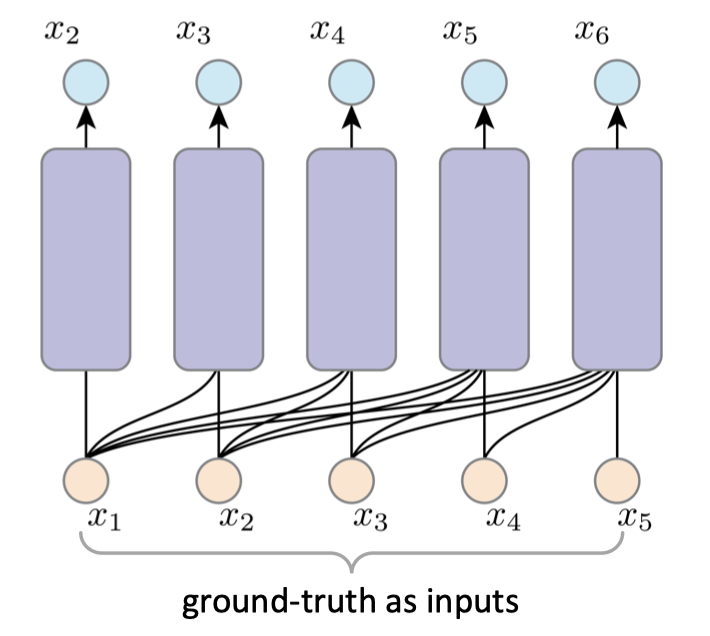
We use a dependency graph to denote this process, shown as below.
 Actually, this dependency graphs reflect the prior knowledge and we can induce numerous versions of the graph, where some of them may induce simpler distributions. Also, conceptually, $x$ can be anything, the raw data or the representation. And it is not necessarily sequential or temporal. These facts are not specific to the autoregressive model.
Here we refer to autoregressive model as a inference-time behavior, where the model uses its own outputs as the inputs for the next predictions, like what GPT does. Usually, it is not affordable to cover all function space without any prior knowledge. If we want to generalize on some kinds of distributions, we need to make assumptions on the predictions. Here the autoregressive model depends on the values in the past, which is an inductive bias. We can leverage such a inductive bias to narrow down the search space of the generative models. Additionally, we want the decomposed distributions to be represented by shared network architectures, although they conceptually have different mappings. Then we have
$$
p(x_{1}, x_{2}, \cdots, x_{n}) = p_{\theta}(x_{1})p_{\theta}(x_{2}|x_{1})\cdots p_{\theta}(x_{n}|x_{1}, x_{2}, \cdots x_{n-1}).
$$
This is made based on the assumption that the statistical features of the sequence is similar at different positions.
Inference in the autoregressive model is straightforward. As for the density estimation, for any arbitrary point $\mathbf{x}$, we compute the log conditions $\log p_{\theta}(x_{i}| x_{<i})$ for each $i$ and then add these up to obtain the log-likelihood assigned by the model to $\mathbf{x}$. Since $\mathbf{x}$ is known, all the conditions can be computed in parallel.
As for the generation, we need to do sampling, which is a sequential procedure. We first sample $x_1$, then we sample $x_2$ conditioned on $x_{1}$, until $x_i$ conditioned on $x_{i-1}$. The sequential sampling can be an expensive process. It is now a hot topic in inference speeding and optimization.
Actually, this dependency graphs reflect the prior knowledge and we can induce numerous versions of the graph, where some of them may induce simpler distributions. Also, conceptually, $x$ can be anything, the raw data or the representation. And it is not necessarily sequential or temporal. These facts are not specific to the autoregressive model.
Here we refer to autoregressive model as a inference-time behavior, where the model uses its own outputs as the inputs for the next predictions, like what GPT does. Usually, it is not affordable to cover all function space without any prior knowledge. If we want to generalize on some kinds of distributions, we need to make assumptions on the predictions. Here the autoregressive model depends on the values in the past, which is an inductive bias. We can leverage such a inductive bias to narrow down the search space of the generative models. Additionally, we want the decomposed distributions to be represented by shared network architectures, although they conceptually have different mappings. Then we have
$$
p(x_{1}, x_{2}, \cdots, x_{n}) = p_{\theta}(x_{1})p_{\theta}(x_{2}|x_{1})\cdots p_{\theta}(x_{n}|x_{1}, x_{2}, \cdots x_{n-1}).
$$
This is made based on the assumption that the statistical features of the sequence is similar at different positions.
Inference in the autoregressive model is straightforward. As for the density estimation, for any arbitrary point $\mathbf{x}$, we compute the log conditions $\log p_{\theta}(x_{i}| x_{<i})$ for each $i$ and then add these up to obtain the log-likelihood assigned by the model to $\mathbf{x}$. Since $\mathbf{x}$ is known, all the conditions can be computed in parallel.
As for the generation, we need to do sampling, which is a sequential procedure. We first sample $x_1$, then we sample $x_2$ conditioned on $x_{1}$, until $x_i$ conditioned on $x_{i-1}$. The sequential sampling can be an expensive process. It is now a hot topic in inference speeding and optimization.
 What about training?
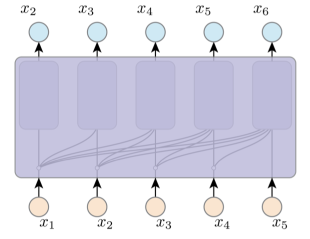
If we obey the dependency graph of the inference, the gradient would be explosive. For example, if we want to compute the gradient of $x_6$, we need to recursively trace its dependency graph to all the previous inputs and sampling operations, and pass all the previous networks. It would be exponentially large and infeasible. To this end, we adopt teacher forcing in the training stage.
Normally, when the model generates $i$-th outputs, the $(i-1)$-th prediction results would be used. However, in teacher forcing, we feed the true labels to the next step.
What about training?
If we obey the dependency graph of the inference, the gradient would be explosive. For example, if we want to compute the gradient of $x_6$, we need to recursively trace its dependency graph to all the previous inputs and sampling operations, and pass all the previous networks. It would be exponentially large and infeasible. To this end, we adopt teacher forcing in the training stage.
Normally, when the model generates $i$-th outputs, the $(i-1)$-th prediction results would be used. However, in teacher forcing, we feed the true labels to the next step.
 In this way, we turn a sequential learning problem into a parallel supervised learning. And the training goal is
$$
L(\theta) = - \sum_{i=1}^{N} \log[p_{\theta}(y_{i}|y_{<i}, x)]
$$
where $y_{<i}$ is the true labels. This brings about several benefits. First, we can avoid the error accumulation. Second, it will speed up the convergence, as we can get more accurate gradient feedback at each step. Intuitively, it resembles the process of looking at the answers when learning from example questions, which will make it faster for us to learn about how to solve the problem. The drawback is clear as well. As we expose the true labels every time and at the inference stage, the models has to rely on its own estimation, which will lead to the inconsistencies in the distributions between training and testing.
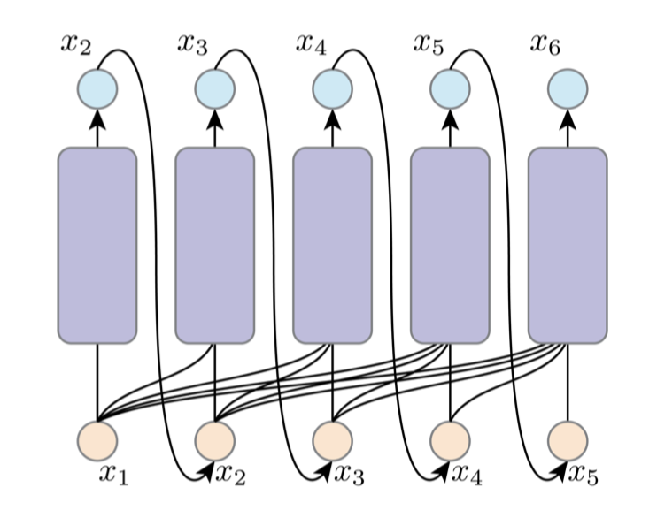
At the same time, as we have introduced the inductive bias, we can implement AR
by one network, with shared arch, weights and computation. To make sure that $x_i$ only sees $x_{<i}$, we can apply masked attention / convolution. It means we filter out the information in the future to ensure the autoregressive features.
In this way, we turn a sequential learning problem into a parallel supervised learning. And the training goal is
$$
L(\theta) = - \sum_{i=1}^{N} \log[p_{\theta}(y_{i}|y_{<i}, x)]
$$
where $y_{<i}$ is the true labels. This brings about several benefits. First, we can avoid the error accumulation. Second, it will speed up the convergence, as we can get more accurate gradient feedback at each step. Intuitively, it resembles the process of looking at the answers when learning from example questions, which will make it faster for us to learn about how to solve the problem. The drawback is clear as well. As we expose the true labels every time and at the inference stage, the models has to rely on its own estimation, which will lead to the inconsistencies in the distributions between training and testing.
At the same time, as we have introduced the inductive bias, we can implement AR
by one network, with shared arch, weights and computation. To make sure that $x_i$ only sees $x_{<i}$, we can apply masked attention / convolution. It means we filter out the information in the future to ensure the autoregressive features.
 Although it is a recursive process, AR model does not necessarily rely on RNN. Instead, it can be any architecture, including RNN, CNN and Transformer.
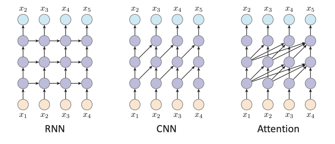 For RNN, every latent is dependent on the previous latent, so it is passed strictly with the order. For CNN, the convolution serves as the sliding windows, so every output is dependent on the regions. For the attention, it allows the output to observe all the history inputs, which is better at global modeling.
Finally, we need to point out that AR models do not directly learn the latent space for unsupervised learning. Therefore, there is no nature ways to get the features. In the next, we will introduce the latent variable models (VAE) which instead explicitly learn the representation of the data.
Variational Autoencoder (VAE)
We have talked about the autogressive model which is modeled as a conditional probality where we represent them as the neural networks. And the cons of the AR models are clear. It requires a ordering, which is usually artificially specified. It is also hard to parallelize when generating. Moreover, it in nature does not support the unsupervised learning for the features.
Variational Autoencoder (VAE) belongs to another paradigm of generative model, a.k.a., latent variable model. The key intuition behind the latent variable model is, instead of modeling the $x$ directly, we model the features of $x$ first. For example, for human facial images, we can tell the age, gender, hair color from them. These latent $z$ are implicitly embedded in the image and can be representative. To this end, we model $p(x|z)$ to generate $x$, which is
$$
p(x) = p(x, z) = \sum_{z}p(z)p(x|z).
$$
Taking image as an example, we basically mask some part of the image and $z$ is unobserved when training. We use the neural network to represent the space.
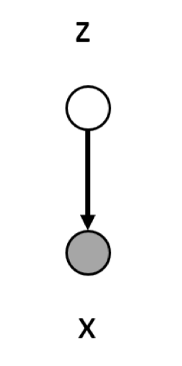 We have a model to model this joint distribution $p(x, z; \theta)$. Given $z \sim N(0, I)$, we model the $p(x|z)$ as $\mathcal{N}(\mu_{\theta}(z), \Sigma_{\theta}(z))$. Then the probability to observe the training data $\hat{x}$ is given by $\sum_z p(\hat{x}, z; \theta)$. How we train the network? Recall the goal of generative learning, which is the maximum likelihood learning, we need to compute
$$
\log p_{\theta}(x) = \sum_{x \in \mathcal{D}} \log p(x; \theta) = \sum_{x \in \mathcal{D}} \log \sum_{z} p(x, z; \theta).
$$
As we can see, $\sum_{z}p(x,z;\theta)$ is intractable, since it is exponentially increased with the size of $z$. So we need to find an alternative way to estimate the value. A straightforward way is to use Monte Carlo sampling, as it is an unbiased estimation as we talk before. However, it does not give us the recipe. The core reason is, $p(x, z)$ is small for most of the cases (imagine most of the completions do not make sense). And it is hardly to “hit” the case when the $p(x, z)$ is maximized. Given this observation, we do not need to randomly sample over all the space. Rather, we can adopt the importance sampling, where we find $q(z)$ as the distribution of $z$. We have
We have a model to model this joint distribution $p(x, z; \theta)$. Given $z \sim N(0, I)$, we model the $p(x|z)$ as $\mathcal{N}(\mu_{\theta}(z), \Sigma_{\theta}(z))$. Then the probability to observe the training data $\hat{x}$ is given by $\sum_z p(\hat{x}, z; \theta)$. How we train the network? Recall the goal of generative learning, which is the maximum likelihood learning, we need to compute
$$
\log p_{\theta}(x) = \sum_{x \in \mathcal{D}} \log p(x; \theta) = \sum_{x \in \mathcal{D}} \log \sum_{z} p(x, z; \theta).
$$
As we can see, $\sum_{z}p(x,z;\theta)$ is intractable, since it is exponentially increased with the size of $z$. So we need to find an alternative way to estimate the value. A straightforward way is to use Monte Carlo sampling, as it is an unbiased estimation as we talk before. However, it does not give us the recipe. The core reason is, $p(x, z)$ is small for most of the cases (imagine most of the completions do not make sense). And it is hardly to “hit” the case when the $p(x, z)$ is maximized. Given this observation, we do not need to randomly sample over all the space. Rather, we can adopt the importance sampling, where we find $q(z)$ as the distribution of $z$. We have
$$ \log p_{\theta}(x) = \log \sum_{x \in \mathcal{D}} p(x; \theta) = \log \sum_{x \in \mathcal{D}}\frac{q(z)}{q(z)} p(x, z; \theta) = \log \mathbb{E}_{z \sim q(z)} \left[\frac{p(x,z; \theta)}{q(z)}\right]. $$
However, it is clear that we still cannot compute this.
Why is that? Think about the above equation. Although we add the importance sampling, we have to integrate in the space of $z$ to compute the expectations, which is usually unrealistic. While Monte Carlo can unbiasedly estimate $\mathbb{E}_{z \sim q(z)} \left[\frac{p(x,z; \theta)}{q(z)}\right]$, it cannot unbiasedly estimate its logarithm. Due to Jensen’s inequality, $\mathbb{E}[\log(\cdot)] \le \log \mathbb{E}[\cdot]$ , so naive Monte Carlo would yield a biased (downward) estimation.
Fortunately, we can compute its lower bound due to the concavity of log function,
$$ \begin{aligned} \log p_{\theta}(x) &= \log \mathbb{E}_{z \sim q(z)} \left[\frac{p(x,z; \theta)}{q(z)}\right] \\ &= \log \sum_{z} q(z) \frac{p(x, z; \theta)}{q(z)} \\ &\ge \sum_{z} q(z)\log \frac{p(x, z; \theta)}{q(z)} \\ &= \mathbb{E}_{z \sim q(z)} \log \left[\frac{p(x,z; \theta)}{q(z)}\right] = \mathrm{ELBO}. \end{aligned} $$
It is Evidence Lower Bound (ELBO). Note that we have no assumptions for $q(z)$, thus it works for any distribution. The ELBO gives us a lower bound of $\log p_{\theta}(x)$. Although we cannot compute its value, we know the minimum value of it. Then maximum likelihood learning would possibly work. A nature question arises here: how tight is the bound and how to choose $q(z)$ to make the bound tight. Luckily, we find that the equality holds when $q(z) = p(z|x; \theta)$. We prove as below.
$$ \begin{aligned} \mathbb{E}_{z \sim q(z)} \log \left[\frac{p(x,z; \theta)}{q(z)}\right] &= \sum_{z} q(z) \log \frac{p(x, z; \theta)}{q(z)} \\ &= \sum_{z} p(z|x; \theta) \log \frac{p(x, z; \theta)}{p(z|x)} \\ &= \sum_{z} p(z|x; \theta) \log \frac{p(z|x; \theta)p(x; \theta)}{p(z|x; \theta)} \\ &= \sum_{z} p(z|x; \theta) \log p(x; \theta) \\ &= \log(p; \theta) \sum_{z} p(z|x; \theta) \\ &= \log(p; \theta). \end{aligned} $$
So, if $q(z)$ matches the completed one, it will lead to the ELBO the same as the log-likelihood. This is a tight bound. Then we take a look at what this bound stands for.
$$ \begin{aligned} \text{ELBO} &= \sum_{z}q(z)\log \frac{p(x, z; \theta)}{q(z)} \\ &= \sum_{z}q(z) \log p(x, z; \theta) - \sum_{z} q(z) \log q(z) \\ &= \sum_{z}q(z) \log p(x, z; \theta) + H(q), \end{aligned} $$
where $H(\cdot)$ is the entropy. We can further compute
$$ \begin{aligned} D_{KL}(q(z) || p(z|x; \theta)) &= \sum_{z} q(z) \log \frac{q(z)}{p(z|x; \theta)}\\ &= -\sum_{z}q(z) \log p(z|x; \theta) - H(q) \\ &= -\sum_{z}q(z) \log \left[\frac{ p(x,z; \theta)}{p(x)}\right] - H(q) \\ &= -\sum_{z}q(z) \log p(x,z; \theta) + \sum_{z}q(z) \log p_{\theta}(x) - H(q) \\ &= -\sum_{z}q(z) \log p(x,z; \theta) + \log p_{\theta}(x) - H(q) \ge 0. \end{aligned} $$
That also explains why the ELBO equality holds when $q(z) = p(z|x; \theta)$. So we can have
$$ \log p_{\theta}(x)= D_{KL}(q(z) || p(z|x; \theta)) + \mathbb{E}_{z \sim q(z)} \log \left[\frac{p(x,z; \theta)}{q(z)}\right] = D_{KL}(q(z) || p(z|x; \theta)) + \text{ELBO}. $$
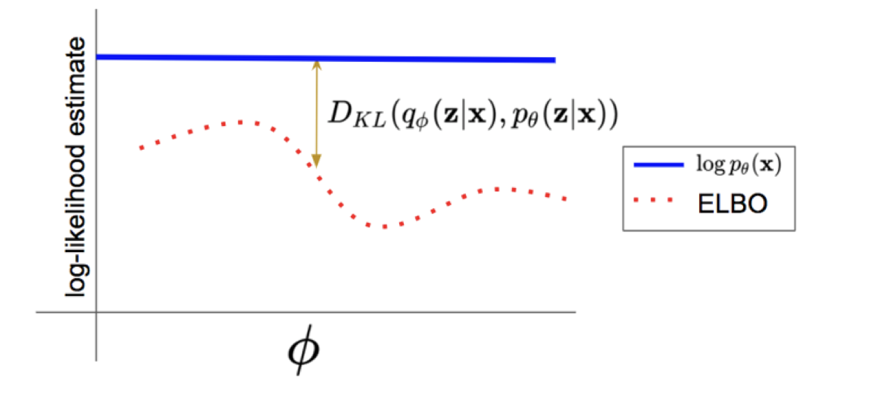 As can be seen from the graph, the ELBO is the lower bound of the log-likellihood. And the difference between them is the KL-divergence. We can easily compute the ELBO, while $D_{KL}(q(z) || p(z|x; \theta))$ and $\log p_{\theta}(x)$ is intractable. However, if $q$ is close to the ground truth, the $D_{KL}(q(z) || p(z|x; \theta))$ will be converged to 0, then the ELBO is an exact approximation of the log-likelihood.
Let’s continue to look at the ELBO. We rewrite the ELBO here. $$ \text{ELBO} = \sum_{z}q(z) \log p(x, z; \theta) - \sum_{z} q(z) \log q(z). $$ $q(z)$ is a universal function that can be any distribution. Then how we can train it? We can parameterize $q(z)$ with $q_{\phi}(z|x)$, where $\phi$ is a neural network.
Recall that $q(z)$ can be any function. Therefore, using $q_{\phi}(z|x)$ will not break the properties of ELBO. Furthermore, as we can tell from the generation problem, the $q$ should be chosen as a completion problem. By conditioning on $x$, it is more reasonable to give $z$ to complete the signal. Note that it is not mathematically the best choice. However, using such parameterization is enough for most of the generative problems and it works well.
Then we can write the loss as
$$ \begin{aligned} L(x, \theta, \phi) &= \sum_{z}q_{\phi}(z|x) \log p(x, z; \theta) - \sum_{z} q_{\phi}(z|x) \log q_{\phi}(z|x)\\ &=\sum_{z}q_{\phi}(z|x) \log [p_{\theta}(x|z)p(z)] - \sum_{z} q_{\phi}(z|x) \log q_{\phi}(z|x)\\ &= \sum_{z}q_{\phi}(z|x) \log p_{\theta}(x|z) - \sum_{z} q_{\phi}(z|x) \log \frac{q_{\phi}(z|x)}{p(z)} \\ &= \mathbb{E}_{z \sim q_{\phi}(z|x)} \log p_{\theta}(x|z) - D_{KL} (q_{\phi}(z|x)||p(z)). \end{aligned} $$
In standard VAE, we use a fixed prior of $p(z)$ and do not parameterize it with the neural network (but we can as well). We will discuss it later.
A typical VAE has the following framework:
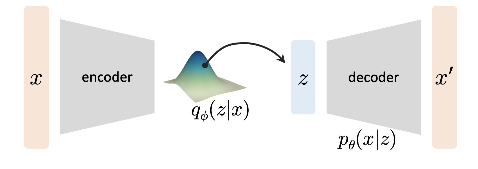 We use an encoder to output the distribution of $q$ and sample $z$ from it. Then we deconstruct from $z$ through a decoder $p_{\theta}(x|z)$. From the above loss, we can tell:
- $\mathbb{E}_{z \sim q_{\phi}(x|z)}\log p_{\theta}(x|z)$ is the reconstruction loss. It measures how close the generated $x$ is with the true sample.
- $D_{KL} (q_{\phi}(z|x)||p(z))$ is the regularization loss. It ensures that $q_{\phi}(z|x)$ is closed to the prior distribution.
$p(z)$ is the prior assumption of $z$. Usually it is a Gaussian distribution. Why do we need $q_{\phi}(z|x)$ to be closed to $p(z)$? When we look at the inference stage, it contains two steps:
- Sample $z$ from $p(z)$: $z \sim p(z)$
- Generate the new data via $p_{\theta}(x|z)$
However, during the training phase, the input of the decoder is $q_{\phi}(z|x)$. Therefore, this loss is crucial to avoid overfit by remembering the latent codes from $q_{\phi}(z|x)$. At the same time, it gives a smooth interpolation of the latent code that can generalize well to the new data.
So basically, our training goal is to optimize two networks: the decoder $p_{\theta}$ and the encoder $q_{\phi}$. And the training is concluded as follows:
- We train $q_\phi(z|x)$ given the $x$
- We sample the latent from $q_{\phi}(z|x)$
- We use the latent to train $p_{\theta}(x|z)$ Here we have a detailed trick. The sampling of $q_{\phi}(z|x)$ is non-differentiable. So we use a reparameterization trick here. We let the network $q_{\phi}(z|x)$ to output two variables: $\mu_{\phi}(x)$ and $\sigma_{\phi}(x)$. Then we use the following sample:
$$ z \sim \mu_{\phi}(x) + \sigma_{\phi}(x) \cdot \epsilon, \epsilon \in \mathcal{N}(0,\mathbf{I}). $$
At the inference stage, we generate the data by the following steps:
- We first sample $z \sim \mathcal{N}(0, \mathbf{I})$
- Then we compute $x \sim p_{\theta}(x|z)$.
So far, we have seen two modeling of generative learning. For AR, the modeling is quite straightforward by utilizing the conditional probability. On the other hand, the latent-based model learns the latent space first and leverages a set of encoder and decoder to reconstruct the data. We will then see other means of the modeling in the subsequent notes.
References
Stanford University CS236: Deep Generative Models MIT 6.S978: Deep Generative Models, Fall 2024 zhuanlan.zhihu.com/p/719118354